What Is a Perceptron? Complete Guide & Examples

Imagine you’re building a spam filter for your email. How does the computer decide whether “Congratulations! You’ve won $1 million!” is spam, while “Meeting moved to 3 PM” is legitimate?

Meet the perceptron: What is a perceptron? It’s the simplest form of an artificial neuron that forms the foundation of modern deep learning. A deceptively humble algorithm that sparked both the greatest optimism and deepest disappointments in AI history. When Frank Rosenblatt first demonstrated his Mark I Perceptron machine at Cornell in 1960, newspapers proclaimed it would soon “walk, talk, see, write, reproduce itself and be conscious of its existence”. Yet within a decade, the limitations of this simple model nearly killed neural network research entirely, something I’ve explored in detail in From AI Spring to AI Winter: A Timeline of Hype, Hope, and Hard Lessons.

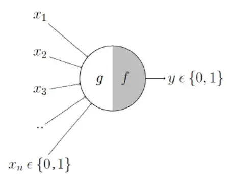
At its core, the Perceptron is one of the simplest machine learning algorithms — essentially a mathematical model inspired by the way neurons work in the brain (read more about this in The Biological Roots of Neural Networks). Imagine a single decision-making unit that mimics a neuron: it takes several inputs, weighs their importance, sums them up, and decides-teaches itself from experience whether to fire (1) or not (0).

The older model of perceptron used to take a bunch of Boolean inputs. If the sum of all inputs crosses a certain threshold, the perceptron outputs one category; otherwise, it outputs the other (often referred to as +1 and -1 or 1 and 0).

Step 1:

\[
g(x) =\sum_{i=1}^{n} x_i \
\]

Step 2:

\[
f(x) =
\begin{cases}
1 & \text{if } g(x) > \theta \\
0 & \text{otherwise}
\end{cases}
\]

For example, let’s say we want to predict whether I would eat a cookie. to answer that, we need some information before making a decision, like:

Am I hungry?
Is it a salty cookie?
Do I like this brand?
Do I have a cookie at home?

(1 for Yes, 0 for No)

There could be more variables that might alter my choice, but for the sake of simplicity, let’s just assume only these 4 are enough for my decision. Now let’s assume our input is [1, 0, 1, 0], which means: I am hungry (1), it’s not a salty cookie (0), I like this brand (1), but I don’t have a cookie at home (0). Now, if the sum of all the inputs is greater than a threshold (Used Step Function as Activation Function), the perceptron returns 1 (That means: Yes, I will eat the cookie). Otherwise, it outputs 0 (No, I won’t eat the cookie).

Limitations

Soon, we realized there were some major problems with the original perceptron model, like the model was giving the same weightage to all the inputs. for example, if I am hungry or not, it might play a more important role in my decision than if I like the brand.

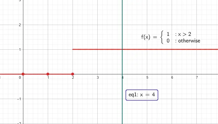
Another issue with the Activation Function. Previously, we were only using the step function, which restricted our view to only 0 and 1. For example, let say there are 100 inputs and assuming the threshold is 50, if the summation of inputs is 49, then our model return -1, and if the summation is incremented just by 1, that is 50, now our model returns +1. which is actually not how we work, even at 49 there is good 50/50 chance to fall under any of the 2 categories.

And one more limitation was that the older perceptron model was designed to only work for a binary classification model. For regression problems, this model was completely useless.

The Modern Perceptron Model

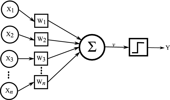
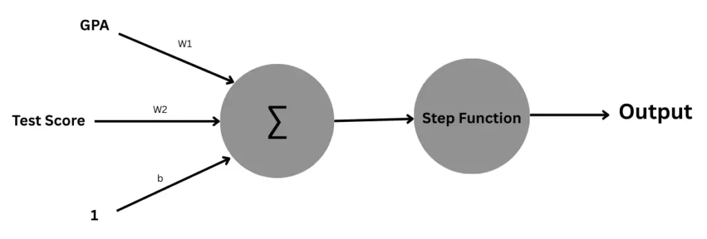
In the modern perceptron model, we are trying to solve all these problems. Starting with weights and bias. As stated before, for the cookie problem, being hungry has more impact than if I like the brand. So now we multiply all the inputs by a weight, which shows how much impact that input was on my decision. Then we calculate the weighted sum of the inputs, and then add bias to show my natural tendency regarding eating a cookie. model.

Step 1:

\[
g(x) = \sum_{i=1}^{n} w_i x_i + b
\]

– $x_i$: the $i^{th}$ input feature
– $w_i$: the weight (importance) associated with input $x_i$
– $b$: the bias term, which shifts the decision boundary
– $n$: the total number of input features
– $g(x)$: the weighted sum (also called the net input)

Step 2:

\[
f(x) =
\begin{cases}
1 & \text{if } g(x) > \theta \\
0 & \text{otherwise}
\end{cases}
\]

– $f(x)$: the perceptron’s final output (0 or 1)
– $g(x)$: the net input (weighted sum of inputs + bias)
– $\theta$: the threshold value that decides the cutoff point

To understand better, let’s continue with our previous example with the new model.

Let’s assign some weights to each input:

Hungry → weight = 2.0
Salty cookie → weight = -1.0 (negative because I don’t like salty cookies)
Like the brand → weight = 1.5
Have a cookie at home → weight = 1.0

And let’s set:

Bias = 0.5
Threshold = 2.0

Bias = 0.5, means: “Even if the inputs are not strong enough, I have a slight tendency to eat cookies.”
If bias = 0, I will only eat a cookie when the inputs alone make the weighted sum cross the threshold.
If bias = -0.5, it’s the opposite: “I’m slightly less likely to eat cookies unless I get strong positive reasons from the inputs.”

Now, our input was [1, 0, 1, 0] → (Hungry = 1, Salty = 0, Like brand = 1, Have cookie = 0).

There are many different types of Activation functions, each having its own Pros and Cons. We’ll soon explore these activation functions in detail, covering how they work, when to use each, and what trade-offs they bring. Stay tuned for upcoming posts diving into gradient behavior, network depth, and multi-layer architectures.

The perceptron calculates:

$Weighted sum = x_{1}w_{1} + x_{2}w_{2} + x_{3}w_{3} + x_{4}w_{4} + b$

Since 4.0 > 2.0 (threshold), the perceptron outputs:

This solved our first problem.

We can also perform the calculation using matrix multiplication. For that, we will pass our inputs as a vector, with an additional 1 at the end of the vector, (Original Input : [1, 0, 1, 0], New Input vector : [1, 0, 1, 0, 1]), and perform a dot product with the modified weight vector, where we also include bias at the end of the vector (Original Weight Vector: [2.0, -1.0, 1.5, 1.0], New Weight Vector: [2.0, -1.0, 1.5, 1.0, 0.5] ). The formula for this looks like this:

\[
z = \tilde{\mathbf{x}}^\top \tilde{\mathbf{w}},
\quad
\tilde{\mathbf{x}} =
\begin{bmatrix}
x_{1}\\ x_{2}\\ \vdots \\ x_{n}\\ 1
\end{bmatrix},\
\tilde{\mathbf{w}} =
\begin{bmatrix}
w_{1}\\ w_{2}\\ \vdots \\ w_{n}\\ b
\end{bmatrix}
\]

Then we apply the Activation Function to the resultant. Let’s look into an actual code implementation:

I highly encourage you to copy this code to your preferred code editor and play around a bit, maybe change the input or weights, what if the threshold is a little low? and let me know how that works.

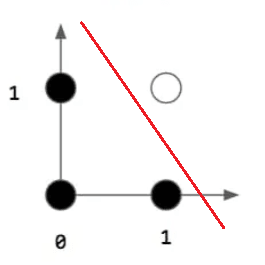
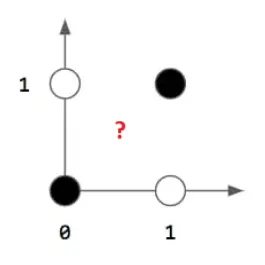
As you can see how it works, but still nowadays, perceptions aren’t used this way. A single perceptron can work perfectly for linearly separable data, but in the real-world scenario, things are not this simple; the majority of data is complex and can’t be separated by a straight line decision boundary, and Perceptrons only work for linearly separable data by creating a straight line decision boundary. For example, it works perfectly for AND and OR operations, but not for XOR. If you are wondering what a decision boundary is, worry not; this is covered in the section below.

AND

Input 1	Input 2	Output
1	1	1
1	0	0
0	1	0
0	0	0

OR

Input 1	Input 2	Output
1	1	1
1	0	1
0	1	1
0	0	0

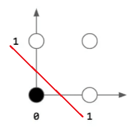
XOR

Input 1	Input 2	Output
1	1	0
1	0	1
0	1	1
0	0	0

🐍

perceptron.py

import numpy as np

class Perceptron:
    """
    A simple perceptron implementation for binary classification.
    """
    
    def __init__(self, threshold=0.0):
        """
        Initialize the perceptron.
        
        Args:
            threshold (float): Decision threshold for activation
        """
        self.threshold = threshold
    
    def _weighted_sum(self, inputs, weights):
        """
        Calculate the weighted sum of inputs.
        
        Args:
            inputs (list/array): Input features including bias term
            weights (list/array): Weights including bias weight
            
        Returns:
            float: Weighted sum
        """
        return np.dot(inputs, weights)
    
    def _step_activation(self, weighted_sum):
        """
        Apply step activation function.
        
        Args:
            weighted_sum (float): Result from weighted sum
            
        Returns:
            int: 1 if activated, 0 otherwise
        """
        return 1 if weighted_sum >= self.threshold else 0
    
    def predict(self, inputs, weights):
        """
        Make a prediction for given inputs.
        
        Args:
            inputs (list/array): Input features including bias term
            weights (list/array): Weights including bias weight
            
        Returns:
            int: Predicted class (0 or 1)
        """
        weighted_sum = self._weighted_sum(inputs, weights)
        return self._step_activation(weighted_sum)

# Example usage with your cookie decision problem
def cookie_decision_example():
    """
    Example: Cookie eating decision using perceptron.
    """
    # Initialize perceptron with threshold of 2.0
    perceptron = Perceptron(threshold=2.0)
    
    # Input features: [hungry, salty, like_brand, have_at_home, bias]
    inputs = [1, 0, 1, 0, 1]
    
    # Weights: [w_hungry, w_salty, w_brand, w_home, bias_weight]
    weights = [2.0, -1.0, 1.5, 1.0, 0.5]
    
    # Make prediction
    prediction = perceptron.predict(inputs, weights)
    
    # Display results
    weighted_sum = np.dot(inputs, weights)
    print(f"Weighted sum: {weighted_sum}")
    print(f"Threshold: {perceptron.threshold}")
    print(f"Prediction: {prediction}")
    print(f"Decision: {'Eat the cookie!' if prediction == 1 else 'Skip the cookie.'}")
    
    return prediction

# Run the example
if __name__ == "__main__":
    cookie_decision_example()

Training a Perceptron

Let’s take another example to understand this. Say, A university uses a simple perceptron to make preliminary admission decisions based on just two factors:

Student’s GPA Score (range: 1-10)
Standardized Test Score (range: 1-100)

As we have already seen how the Perceptron will work to find the output, but you might have an obvious question: we have the given input data, that’s ok, but what about the weights and bias? how would we know the weights and bias? So let me tell you, this is the whole problem that we don’t know already what what should be the values of Weights and bias should be, and this is exactly what we try to find while training the perceptron. These types of variables are called Hyperparameters. Think of your grandfather’s radio, if you want to listen to some music or maybe your favorite host is live, to get to the channel, you rotate the knob, in the hope of getting to the desired channel and even if you reach to the channel sound might not be very good, as there could be a lot of white noise, so you adjust the antenna. Yeah!! It was challenging back in the day, but what I am trying to explain is how we worked with the radio, rotating the knob and adjusting the antenna in the direction for better sound quality, and finding a sweet spot where it provided the best sound for you. We do the same with Perceptron Hyperparameters.

Let’s have a look at last year’s student admissions dummy data. We want to train our perceptron model (meaning find the best weights and bias), based on this data, so that it can decide whether the new student should be admitted or not:

GPA	TestScore	Admit
4.4	97.0	1
9.6	78.0	1
7.6	94.0	1
6.4	90.0	0
2.4	60.0	0
2.4	92.0	0
1.5	10.0	0
8.8	20.0	0
6.4	5.0	0
7.4	33.0	0
1.2	39.0	0
9.7	28.0	1
8.5	83.0	1
2.9	36.0	0
2.6	29.0	0
2.7	55.0	0
3.7	15.0	0
5.7	80.0	0
4.9	8.0	0
3.6	99.0	0
6.5	77.0	1
2.3	21.0	0
3.6	2.0	0
4.3	82.0	0
5.1	71.0	0
8.1	73.0	1
2.8	77.0	0
5.6	8.0	0
6.3	36.0	0
1.4	12.0	0
6.5	86.0	1
2.5	63.0	0
1.6	34.0	0
9.5	7.0	0
9.7	32.0	0
8.3	33.0	0
3.7	73.0	0
1.9	64.0	0
7.2	89.0	1
5.0	48.0	0
2.1	13.0	0
5.5	72.0	0
1.3	76.0	0
9.2	57.0	1
3.3	77.0	0
7.0	50.0	0
3.8	53.0	0
5.7	43.0	0
5.9	4.0	0
2.7	12.0	0

Now let’s create a scatter plot for this data. To do that, you may copy my Python code and run it in your preferred code editor.

🐍

scatter_plot_1.py

import pandas as pd
import matplotlib.pyplot as plt

# --- Using CSV file ---

# Load data from CSV, specify your actual path below
df = pd.read_csv("path_to_your_csv_file.csv")

# Scatter plot for all students (default marker)
plt.scatter(df['GPA'], df['TestScore'])

# Separate admitted and not admitted for different markers/colors
admitted = df[df['Admit'] == 1]
not_admitted = df[df['Admit'] == 0]

# Plot admitted students as green dots 'o'
plt.scatter(admitted['GPA'], admitted['TestScore'], marker='o', color='green', label='Admitted')

# Plot not admitted students as red crosses 'x'
plt.scatter(not_admitted['GPA'], not_admitted['TestScore'], marker='x', color='red', label='Not Admitted')

# Add axis labels and title
plt.xlabel('GPA')
plt.ylabel('Test Score')
plt.title('Student Admission Scatter Plot')

# Show legend
plt.legend()

# Display plot
plt.show()

You can use this code, just replace the ‘path_to_your_csv_file.csv‘ with the path to your CSV file. You may download the dummy data that I used from the download button above.

Alternatively, you may use the code below to create your own random dummy data of your preferred sample size, using Python’s nympy library. Numpy gives you the ability to adjust he data to your needs, you can balance or imbalance any feature as you desire. It’s a very powerful tool; further discussion on numpy is out of the scope of this article, but you should definitely have a look at this, if you don’t already know.

🐍

scatter_plot_2.py

import numpy as np
import matplotlib.pyplot as plt

# Function to generate dummy student admission data and plot
def plot_random_student_admission(sample_size=50, admit_ratio=0.2):
    np.random.seed(42)  # reproducible results

    # Generate random GPA between 1-10
    gpa = np.round(np.random.uniform(1, 10, sample_size), 1)

    # Generate random TestScore between 1-100
    test_score = np.round(np.random.uniform(1, 100, sample_size), 0)

    # Create Admit labels: Set 'admit_ratio' percent as admitted randomly
    admit_labels = np.zeros(sample_size, dtype=int)
    admit_indices = np.random.choice(sample_size, int(admit_ratio * sample_size), replace=False)
    admit_labels[admit_indices] = 1

    # Plot admitted students
    plt.scatter(gpa[admit_labels == 1], test_score[admit_labels == 1], c='green', marker='o', label='Admitted')

    # Plot not admitted students
    plt.scatter(gpa[admit_labels == 0], test_score[admit_labels == 0], c='red', marker='x', label='Not Admitted')

    # Axis labels and plot title
    plt.xlabel('GPA')
    plt.ylabel('Test Score')
    plt.title(f'Student Admission Scatter Plot ({sample_size} samples, {int(admit_ratio*100)}% admitted)')

    # Legend and plot
    plt.legend()
    plt.show()

# Example usage:
plot_random_student_admission(sample_size=30, admit_ratio=0.3)

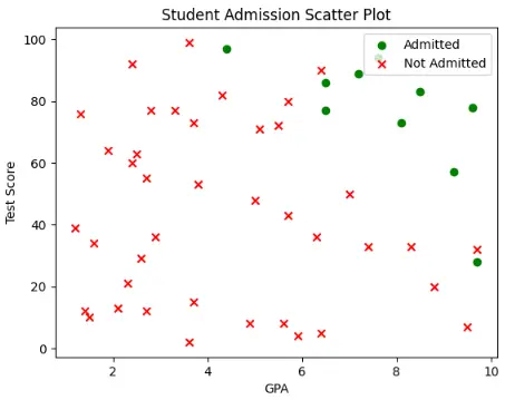
Nonetheless, this is the Scatter Plot of my dummy data that I have shown above. Each point in the graph represents a student; the red cross indicates that the student was not admitted, while the green dot indicates that they were admitted. Now, can we draw a straight line that can segregate the data into admitted and non-admitted students, so that when a new student comes, by looking into their GPA and Test score, we can decide whether they should be admitted or not (We call in this line as Decision Boundary in technical terms), as we learned from earlier admissions? Maybe yes, since we are conscious and smart beings, but it would still challenge me to know which line is the best. Let’s look into these scenarios in fig-9, fig-10, and fig-11. They all divide the graph into 2 regions: a positive region that is at the right-hand side of the decision boundary, and a negative region at the left-hand side.

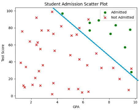
Here, all the admitted students are in the positive regions, but some non-admitted students as also in the positive region, which means they are labelled wrong.

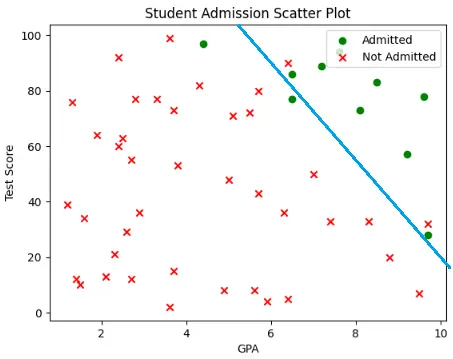
Here, we adjusted the decision boundary so that one of the wrong-labelled non-admitted students is now on the correct side, that is, in the negative region, but 2 of the admitted students also got mislabelled.

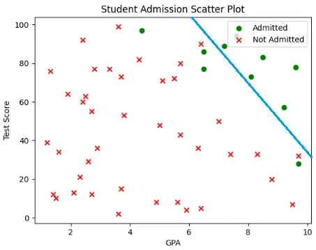
Now we have moved the decision boundary more to the top-right side, so that all the non-admitted students are now in their correct region, that is, the negative region, but some admitted students are again in the wrong region.

So, as you saw, it’s not as easy as it seems. So, how would we solve this? It’s impossible to draw a straight line that will perfectly classify the data into 2 regions, so try to build a confidence level for our decision boundaries by minimizing the errors. There are multiple ways to do that. One of the most common perceptron training models is the Perceptron learning Rule, also known as PLA. We will cover PLA in another blog; just know that, with the help of PLA, we can train our Perceptron model to minimize the errors, and if we use multiple such perceptrons, stacked together in layers, we can create something called a Multi-Layer Perceptron (MLP). With the help of MLP, we are not restricted to a straight line, but can now create a curved line with any level of precision, if we use enough perceptions. All this will be covered in the upcoming blog.

Activation Functions

Now, let’s revisit activation functions. Earlier, we showed how the simple step function limited the perceptron to binary outputs, either 0 or 1, with no notion of confidence or probability.

Modern alternatives unlock much more power:

Sigmoid squashes input to $(0, 1)$ , enabling binary classification with probabilistic interpretation.
Softmax generalizes this to multiple classes, producing a probability distribution across them.
ReLU, Tanh, LELU, and others introduce useful non-linearity, allowing networks to model complex, real-world patterns.

These functions aren’t just mathematical variations, they help networks learn better, generalize, and train efficiently using gradient-based methods.

Sigmoid squashes input to $(0, 1)$ , enabling binary classification with probabilistic interpretation.
Softmax generalizes this to multiple classes, producing a probability distribution across them.
ReLU, Tanh, LELU, and others introduce useful non-linearity, allowing networks to model complex, real-world patterns.

These functions aren’t just mathematical variations, they help networks learn better, generalize, and train efficiently using gradient-based methods.

Quick Activation Summary

Activation Function	Formula	Range	Where It’s Used
Step	\[ f(x) = \begin{cases} 0, & x < \theta \\ 1, & x \geq \theta \end{cases} \]	{0,1}	Early perceptron, binary classification.
Sigmoid	\[ \sigma(x) = \frac{1}{1 + e^{-x}} \]	(0,1)	Binary classification (logistic regression).
Softmax	\[ \sigma(\mathbf{z})_i = \frac{e^{z_i}}{\sum_{j=1}^{K} e^{z_j}}, \quad i = 1, 2, \dots, K \]	(0,1), sums to 1 across classes	Multi-class classification output layers.
Relu	\[ f(x) = \max(0, x) \]	[0,∞)	Hidden layers in deep networks
Tanh	\[ \tanh(x) = \frac{e^x - e^{-x}}{e^x + e^{-x}} \]	(−1,1)	Hidden layers when centered outputs are preferred.
Linear	\[ f(x) = x \]	(−∞,∞)	Regression tasks (continuous output).

Now that you understand how perceptrons work, here’s a challenge: Can you modify the student admission example to include a third factor, like extracurricular activities? How would this change your decision boundary?

Remember, every expert was once a beginner. The concepts you’ve learned here: weighted inputs, activation functions, and decision boundaries, form the foundation of neural networks powering everything from image recognition to language models.

Keep experimenting, keep learning, and most importantly, keep building!

What will you create with your newfound perceptron knowledge?